Extended guide¶

First, load some data:

from ephysiopy.io.recording import AxonaTrial
from pathlib import Path

data = Path("/path/to/data/M851_140908t2rh.set")

trial = AxonaTrial(data)

Trial settings¶

At this point the only data that has been loaded is the settings data. For Axona data this consists of the key - value pairs in the .set file, essentially the state machine of the recording. Because of it's simple structure this is stored as a standard python dictionary

type(trial.settings)
dict

Because of the more flexible/ complex design of the OpenEphys plugin-GUI this settings data is stored as it's own class:

from ephysiopy.io.recording import OpenEphysBase

data = Path("/path/to/data/RHA1-00064_2023-07-07_10-47-31")

trial = OpenEphysBase(data)

type(trial.settings)
ephysiopy.openephys2py.OESettings.Settings

See OEPlugins for more details

You won't need to interact with the settings directly for most if not all analyses; the relevant bits are extracted and used in loading/ processing of other data.

Position data¶

Regardless of the data source, position data is stored in the PosCalcsGeneric class:

trial.load_pos_data()
Loaded pos data

type(trial.PosCalcs)
ephysiopy.common.ephys_generic.PosCalcsGeneric

There are several arguments you can add to the load_pos_data function to control how the position data is treated. An important one is 'ppm' which stads for pixels_per_metre. It specifies how many pixels in camera units correspond to one metre. This is something you should measure experimentally and record somewhere. The number is used to convert the position data to real world units. If you don't specify it, the ppm value will take a default value of 300 (CHECK)

trial.load_pos_data(ppm=800)
Loaded pos data

Other important arguments are jumpmax and cm. Jumpmax is the maximum distance that the animal can move between two frames. If the distance between two frames is greater than this value, the position data for that frame will be interpolated over. This is useful for removing artefacts in the position data caused by tracking errors. The default value is 100 pixels. 'cm' is a boolean that specifies whether the position data should be converted to centimetres. The default value is False, which means that the position data will be in metres.

Once loaded the PosCalcs attribute has several attributes itself like 'xy' and 'dir' which are the x and y position and the head direction.

You shouldn't need to interact with the PosCalcs class directly for most analyses, but it's there if you need it.

The position data is used in several of the plotting functions and in the rate map calculations.

import matplotlib.pylab as plt

trial.plot_spike_path()
plt.show()

Spiking data¶

We can get the spike times in seconds at which a cluster fired:

trial.get_spike_times(2, 3)
masked_array(data=[0.7710416666666666, 4.6870416666666666,
                   4.693291666666667, ..., 2394.8471458333333,
                   2394.8537291666667, 2394.860708333333],
             mask=[False, False, False, ..., False, False, False],
       fill_value=1e+20)

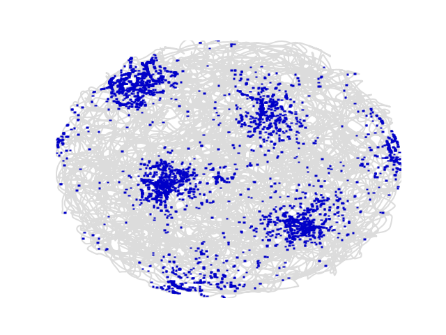
You can plot the position at which spikes were emitted for a specific cluster on top of the path:

trial.plot_spike_path(2, 3)
plt.show()

And the corresponding rate map:

trial.plot_rate_map(2, 3)
plt.show()

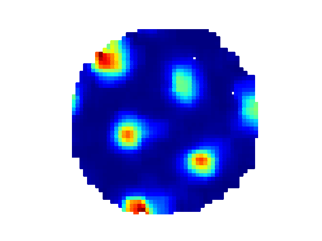
You can access the underlying data for the rate map as well:

trial.get_rate_map(2, 3)

BinnedData(variable=<VariableToBin.XY: 1>, map_type=<MapType.RATE: 1>, binned_data=[masked_array(
...

Read more about the BinnedData class in the API docs BinnedData class and a more verbose description here

Local field potential (LFP) data¶

Load the LFP data like so:

trial.load_lfp()

This can take a while especially if the trial is long and recorded using OpenEphys as the raw data has to be bandpass filtered first. Once that's done the data is available as an EEGCalcs attribute of the trial object

The default sampling rate for the LFP data is 250 Hz, but this can be changed by specifying the 'resample' argument in the load_lfp() function. For example, to resample the LFP data to 500 Hz:

trial.load_lfp(target_sample_rate=500)

Target sample rates should not exceed the Nyquist frequency of the original data, which is half the original sampling rate. For example, if the original sampling rate is 1000 Hz, the target sample rate should not exceed 500 Hz.

Once the data has been loaded you can then bandpass filter it using butterFilter function:

trial.LFP.butterFilter(6, 12)

Filtering a trial¶

There is an apply_filter() method of the trial object that takes a list of TrialFilter and applies those filters to the underlying data of the trial.

Specify a TrialFilter like so:

from ephysiopy.common.utils import TrialFilter

speed_filter = TrialFilter("speed", 0, 5)
trial.apply_filter([speed_filter])

This will filter out all data points where the animal's speed was below 5 cm/s. The filter is applied to all relevant data, so for example the spike times will be masked for all spikes that occurred when the animal was below the speed threshold.

You can build up a list of filters and apply them all at once:

speed_filter = TrialFilter("speed", 0, 5)
time_filter = TrialFilter("time", 100, 200)
trial.apply_filter([speed_filter, time_filter])

The trial has now been filtered for all data points where the animal's speed was below 5 cm/s and where the time was between 100 and 200 seconds. The spike times will be masked for all spikes that occurred when the animal was below the speed threshold or outside the specified time range.

To remove the filters just call the apply_filter() method with no arguments:

trial.apply_filter()

All of the TrialFilter objects take the same arguments: the name of the filter, the minimum value and the maximum value. The name of the filter should be one of the following:

time
dir
speed
xrange
yrange
phi

Examining individual firing fields¶

We can extract individual firing fields from a firing rate map to look more closely at what's happening during individual passes through a firing field.

field_props = trial.get_field_properties(2, 3)
Field 1 has 47 potential runs
Field 2 has 134 potential runs
Field 3 has 165 potential runs
Field 4 has 55 potential runs
Field 5 has 95 potential runs
Field 6 has 113 potential runs
Field 7 has 4 potential runs

The get_field_properties() method has detected 7 fields and a number of runs through each one and returned them as a list.

You can plot the results of this image segmentation like so:

from ephysiopy.common.fieldcalcs import plot_field_props
plot_field_props(field_props)
plt.show()

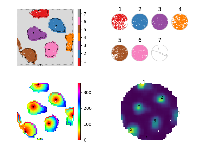
The top left-hand part of the figure shows the results of the segmentation colour-coded for field number (should go from 1 to n numbering from the top left and rastering left to right). The plot at the top-right is the result of taking each run through a field and transforming it so that it lies on a unit circle. This is useful for performing phase precession anaylsis in 2D environments¹. The bottom left-hand part of the figure shows the angle of each point on the perimeter of each field that that firing fields peak and the central heatmap part of each field shows the distance of each bin the field to the firing field centre. The bottom right-hand part of the figure shows the firing rate map numbered with the firing field identity.

There are two important options we can use to change how the extraction of fields from the rate map occurs. The partitioning of the rate map can be done in either a 'simple' or a 'fancy' way.

field_props = trial.get_field_properties(2, 3, partition='simple')

The simple_parition method essentially just returns the areas of the ratemap that are greater than some threshold percentage of the mean firing rate. This was done mostly to deal with one-dimensional linear track data

The fancy_partition method is more complicated in that it will do more image processing under the hood to extract out the relevant areas of the firing rate map. As with the simple method this one only examines areas above some threshold (field_threshold_percent); a local threshold is then applies to each detected sub-field (using skimage.filters.threshold_local). Various metrics are hen extracted and returned to the user.

Each item in field_props in the example above is of type FieldProps and has a large number of attributes availabale. You can also add LFP data for each run through the field(s) which should make phase precession type anaylses easier.

Each field will have one or more runs associated with it, each of these is of type RunProps and has a large number of attributes available.

You can also add LFP data for each run through a field - each run will also then have an LFPSegment object associated with it which contains the LFP data for that run.

Dealing with field properties¶

There are a number of methods for dealing with the field properties objects and their attributes. Because each FieldProps object inherits from the RegionProperties within skimage there is a huge range of attributes available; see https://scikit-image.org/docs/stable/api/skimage.measure.html#skimage.measure.regionprops for a full list.

There are also neuro-specific attrbiutes that are added such as the number of spikes within a field, the phase of theta at which a spike was emitted etc.

It's possible you might want to sort fields by some particular attribute or filter them somehow. As each FieldProps object will have a list of RunProps associated with it it's likely that not all of these runs will have spikes associated with them for example. We may also want to filter out small fields that are unlikely to contain enough data.

from ephysiopy.common.fieldcalcs import sort_fields_by_attr
sorted_fields = sort_fields_by_attr(field_props, "area")
for field in sorted_fields:
    print(field.area)
157.0
132.0
130.0
123.0
100.0
83.0
5.0

We can also filter the runs by some attribute but we need to give a bit more information this time.

from ephysiopy.common.fieldcalcs import filter_runs

filter_runs(field_props, ["num_spikes"], [np.greater], [3])
Filtering runs for n_spikes greater than 3...
Field 1 has 18 potential runs
Filtering runs for n_spikes greater than 3...
Field 2 has 37 potential runs
Filtering runs for n_spikes greater than 3...
Field 3 has 39 potential runs
...    

Notice how the filtering occurs in place so the field_props object is updated with the filtered runs. In this example we have filtered out all runs that had 3 or fewer spikes in them.