Plotting functions
All of these plotting functions are part of a mixin class that is available to OpenEphysBase and AxonaTrial via the base class TrialInterface.
Many of the plotting functions that are part of the FigureMaker class accept keyword arguments that can modify the output. These include:
- separate_plots (bool) - if True and there is more than one cluster & channel given to the method then each one will be plotted in a separate figure. Default is False
- equal_axes (bool) - Make the axes equal or not. Default is True
- cmap (matplotlib.colormaps) - the colormap to use. Mostly this defaults to matplotlib.colormaps['jet']
- ax - matplotlib.Axes instance. If provided the plot will be added to this axis
Some examples:
from ephysiopy.io.recording import AxonaTrial
from pathlib import Path
import matplotlib.pylab as plt

data = Path("/path/to/data/M851_140908t2rh.set")

trial = AxonaTrial(data)
trial.load_pos_data()

trial.plot_rate_map([2,5],[3,3],separate_plots=True,cmap=matplotlib.colormaps['bone'])
plt.show()
ephysiopy.visualise.plotting.FigureMaker()
Bases: object
A mixin class for TrialInterface that deals solely with producing graphical output.
Methods:
| Name | Description |
|---|---|
plot_spike_path |
Plots the spikes on the path for the specified cluster(s) and channel. |
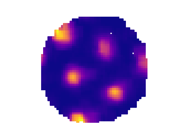
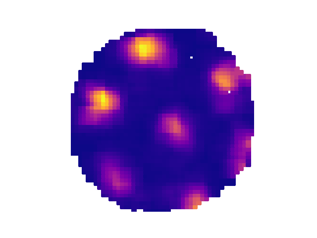
plot_rate_map |
Plots the rate map for the specified cluster(s) and channel. |
plot_hd_map |
Gets the head direction map for the specified cluster(s) and channel. |
plot_linear_rate_map |
Plots the linear rate map for the specified cluster(s) and channel. |
plot_eb_spikes |
Plots the ego-centric boundary spikes for the specified cluster(s) |
plot_eb_map |
Plots the ego-centric boundary map for the specified cluster(s) and |
plot_acorr |
Plots the autocorrelogram for the specified cluster(s) and channel. |
plot_xcorr |
Plots the temporal cross-correlogram between cluster_a and cluster_b |
plot_sac |
Plots the spatial autocorrelation for the specified cluster(s) and channel. |
plot_speed_v_hd |
Plots the speed versus head direction plot for the specified cluster(s) and channel. |
plot_raster |
Plots the raster plot for the specified cluster(s) and channel. |
plot_speed_v_rate |
Plots the speed versus rate plot for the specified cluster(s) and |
plot_power_spectrum |
Plots the power spectrum. |
plot_theta_vs_running_speed |
Plots theta frequency versus running speed. |
plot_clusters_theta_phase |
Plots the theta phase for the specified cluster and channel. |
plot_waveforms |
Plot the waveforms for the selected cluster on the channel (tetrode) |
plotSpectrogramByDepth |
Plots a heat map spectrogram of the LFP for each channel. |
plot_spike_path(cluster=None, channel=None, **kws) -> plt.Axes
Plots the spikes on the path for the specified cluster(s) and channel.
Parameters:
| Name | Type | Description | Default |
|---|---|---|---|
cluster
|
int or None
|
The cluster(s) to get the spike path for. |
None
|
channel
|
int or None
|
The channel number. |
None
|
**kws
|
dict
|
Additional keyword arguments for the function. |
{}
|
Returns:
| Type | Description |
|---|---|
Axes
|
The axes containing the spike path plot. |
plot_rate_map(cluster: int | list, channel: int | list, **kwargs) -> plt.Figure
Plots the rate map for the specified cluster(s) and channel.
Parameters:
| Name | Type | Description | Default |
|---|---|---|---|
cluster
|
int or list
|
The cluster(s) to get the rate map for. |
required |
channel
|
int or list
|
The channel number. |
required |
**kwargs
|
dict
|
Additional keyword arguments for the function. ax : plt.Axes, optional The axes to plot on. If None, new axes are created. separate_plots : bool, optional If True, each cluster will be plotted on a separate plot. Defaults to False. |
{}
|
Returns:
| Type | Description |
|---|---|
Axes
|
The axes containing the rate map plot. |
plot_hd_map(cluster: int, channel: int, **kwargs) -> plt.Axes
Gets the head direction map for the specified cluster(s) and channel.
Parameters:
| Name | Type | Description | Default |
|---|---|---|---|
cluster
|
int
|
The cluster(s) to get the head direction map for. |
required |
channel
|
int
|
The channel number. |
required |
**kwargs
|
dict
|
Additional keyword arguments for the function. |
{}
|
Returns:
| Type | Description |
|---|---|
Axes
|
The axes containing the head direction map plot. |
Notes
NB Following mathmatical convention, 0/360 degrees is 3 o'clock, 90 degrees is 12 o'clock, 180 degrees is 9 o'clock and 270 degrees
plot_linear_rate_map(cluster: int | list, channel: int | list, **kwargs) -> plt.Figure
Plots the linear rate map for the specified cluster(s) and channel.
Parameters:
| Name | Type | Description | Default |
|---|---|---|---|
cluster
|
int or list
|
The cluster(s) to get the linear rate map for. |
required |
channel
|
int or list
|
The channel number. |
required |
**kwargs
|
dict
|
Additional keyword arguments for the function. |
{}
|
Returns:
| Type | Description |
|---|---|
Axes
|
The axes containing the linear rate map plot. |
plot_eb_spikes(cluster: int, channel: int, **kwargs) -> plt.Axes
Plots the ego-centric boundary spikes for the specified cluster(s) and channel.
Parameters:
| Name | Type | Description | Default |
|---|---|---|---|
cluster
|
int
|
The cluster(s) to get the ego-centric boundary spikes for. |
required |
channel
|
int
|
The channel number. |
required |
**kwargs
|
dict
|
Additional keyword arguments for the function. |
{}
|
Returns:
| Type | Description |
|---|---|
Axes
|
The axes containing the ego-centric boundary spikes plot. |
plot_eb_map(cluster: int, channel: int, **kwargs) -> plt.Axes
Plots the ego-centric boundary map for the specified cluster(s) and channel.
Parameters:
| Name | Type | Description | Default |
|---|---|---|---|
cluster
|
int
|
The cluster(s) to get the ego-centric boundary map for. |
required |
channel
|
int
|
The channel number. |
required |
**kwargs
|
dict
|
Additional keyword arguments for the function. |
{}
|
Returns:
| Type | Description |
|---|---|
Axes
|
The axes containing the ego-centric boundary map plot. |
plot_acorr(cluster: int, channel: int, **kwargs) -> plt.Axes
Plots the autocorrelogram for the specified cluster(s) and channel.
Parameters:
| Name | Type | Description | Default |
|---|---|---|---|
cluster
|
int
|
The cluster(s) to get the autocorrelogram for. |
required |
channel
|
int
|
The channel number. |
required |
**kwargs
|
dict
|
Additional keyword arguments for the function, including: binsize : int, optional The size of the bins in ms. Gets passed to SpikeCalcsGeneric.xcorr(). Defaults to 1. |
{}
|
Returns:
| Type | Description |
|---|---|
Axes
|
The axes containing the autocorrelogram plot. |
plot_xcorr(cluster_a: int, channel_a: int, cluster_b: int, channel_b: int, **kwargs) -> plt.Axes
Plots the temporal cross-correlogram between cluster_a and cluster_b
Parameters:
| Name | Type | Description | Default |
|---|---|---|---|
cluster_a
|
int
|
first cluster |
required |
channel_a
|
int
|
first channel |
required |
cluster_b
|
int
|
second cluster |
required |
channel_b
|
int
|
second channel |
required |
Returns:
| Type | Description |
|---|---|
Axes
|
The axes containing the cross-correlogram plot |
plot_sac(cluster: int, channel: int, **kwargs) -> plt.Axes
Plots the spatial autocorrelation for the specified cluster(s) and channel.
Parameters:
| Name | Type | Description | Default |
|---|---|---|---|
cluster
|
int
|
The cluster(s) to get the spatial autocorrelation for. |
required |
channel
|
int
|
The channel number. |
required |
**kwargs
|
dict
|
Additional keyword arguments for the function. |
{}
|
Returns:
| Type | Description |
|---|---|
Axes
|
The axes containing the spatial autocorrelation plot. |
plot_speed_v_hd(cluster: int, channel: int, **kwargs) -> plt.Axes
Plots the speed versus head direction plot for the specified cluster(s) and channel.
Parameters:
| Name | Type | Description | Default |
|---|---|---|---|
cluster
|
int
|
The cluster(s) to get the speed versus head direction plot for. |
required |
channel
|
int
|
The channel number. |
required |
**kwargs
|
dict
|
Additional keyword arguments for the function. |
{}
|
Returns:
| Type | Description |
|---|---|
Axes
|
The axes containing the speed versus head direction plot. |
plot_raster(cluster: int, channel: int, **kwargs) -> plt.Axes
Plots the raster plot for the specified cluster(s) and channel.
Parameters:
| Name | Type | Description | Default |
|---|---|---|---|
cluster
|
int
|
The cluster(s) to get the raster plot for. |
required |
channel
|
int
|
The channel number. |
required |
**kwargs
|
dict
|
Additional keyword arguments for the function, including: dt : list The range in seconds to plot data over either side of the TTL pulse. seconds_per_bin : float The number of seconds per bin. |
{}
|
Returns:
| Type | Description |
|---|---|
Axes
|
The axes containing the raster plot. |
plot_speed_v_rate(cluster: int, channel: int, **kwargs) -> plt.Axes
Plots the speed versus rate plot for the specified cluster(s) and channel.
By default the distribution of speeds will be plotted as a twin axis. To disable set add_speed_hist = False
Parameters:
| Name | Type | Description | Default |
|---|---|---|---|
cluster
|
int
|
The cluster(s) to get the speed versus rate plot for. |
required |
channel
|
int
|
The channel number. |
required |
**kwargs
|
dict
|
Additional keyword arguments for the function. |
{}
|
Returns:
| Type | Description |
|---|---|
Axes
|
The axes containing the speed versus rate plot. |
plot_power_spectrum(**kwargs) -> plt.Axes
Plots the power spectrum.
Parameters:
| Name | Type | Description | Default |
|---|---|---|---|
**kwargs
|
Additional keyword arguments passed to _getPowerSpectrumPlot |
{}
|
plot_theta_vs_running_speed(**kwargs) -> plt.Axes
Plots theta frequency versus running speed.
Parameters:
| Name | Type | Description | Default |
|---|---|---|---|
**kwargs
|
dict
|
Additional keyword arguments for the function, including: low_theta : float The lower bound of the theta frequency range (default is 6). high_theta : float The upper bound of the theta frequency range (default is 12). low_speed : float The lower bound of the running speed range (default is 2). high_speed : float The upper bound of the running speed range (default is 50). |
{}
|
Returns:
| Type | Description |
|---|---|
QuadMesh
|
The QuadMesh object containing the plot. |
plot_clusters_theta_phase(cluster: int, channel: int, **kwargs) -> plt.Axes
Plots the theta phase for the specified cluster and channel.
Parameters:
| Name | Type | Description | Default |
|---|---|---|---|
cluster
|
int
|
The cluster to get the theta phase for. |
required |
channel
|
int
|
The channel number. |
required |
**kwargs
|
dict
|
Additional keyword arguments for the function. |
{}
|
Returns:
| Type | Description |
|---|---|
Axes
|
The axes containing the theta phase plot. |
plot_waveforms(cluster: int, channel: int, **kws) -> list[plt.Axes]
plotSpectrogramByDepth(nchannels: int = 384, nseconds: int = 100, maxFreq: int = 125, channels: list = [], frequencies: list = [], frequencyIncrement: int = 1, **kwargs)
Plots a heat map spectrogram of the LFP for each channel. Line plots of power per frequency band and power on a subset of channels are also displayed to the right and above the main plot.
Parameters:
| Name | Type | Description | Default |
|---|---|---|---|
nchannels
|
int
|
The number of channels on the probe. |
384
|
nseconds
|
int
|
How long in seconds from the start of the trial to do the spectrogram for (for speed). Default is 100. |
100
|
maxFreq
|
int
|
The maximum frequency in Hz to plot the spectrogram out to. Maximum is 1250. Default is 125. |
125
|
channels
|
list
|
The channels to plot separately on the top plot. |
[]
|
frequencies
|
list
|
The specific frequencies to examine across all channels. The mean from frequency: frequency+frequencyIncrement is calculated and plotted on the left hand side of the plot. |
[]
|
frequencyIncrement
|
int
|
The amount to add to each value of the frequencies list above. |
1
|
**kwargs
|
dict
|
Additional keyword arguments for the function. Valid key value pairs: "saveas" - save the figure to this location, needs absolute path and filename. |
{}
|
Notes
Should also allow kwargs to specify exactly which channels and / or frequency bands to do the line plots for.